Introducing realtR

Alex Bresler 2018-03-28

The United States residential real estate brokerage industry is one of the slimiest, shadiest, misaligned industries in existence.

Brokers lie, hoard information, and generally do what it takes to serve their best interests, a commission check.

Often times, a broker aggressively attempts to tricks an individual into engaging them as what is known as a “dual-agent” an agent that represents both a buyer an a seller. They do this to collect a DOUBLE commission while not honestly serving either party.

Worsening matters, the brokerage industry is an extremely organized, political connected cartel that inserts itself into any situation jeopardizing their intermediary role.

This current state has created a number of externalities including:

Stifled innovation

Decreased efficiency

Inflated prices

Changing all that is wrong with this industry is no easy task, but I am optimistic that innovation and serving the customer’s best interests will eventually win out.

Why I Built realtR

There is an old saying, Talk is Cheap.

I often complain about the real estate brokerage industry but outside of a few seed stage investments I haven’t done much about about it.

It’s my hope that realtR is a small step towards a more transparent real estate industry that I personally influenced.

With a bit of R skills, anyone has access to reservoirs of real estate information for EVERY market in the states.

This may sound like a broker-esque promise, all fluff and no substance, but as you will soon see, realtR gives you Real Estate Super Powers.

Also, I enjoy creating sharable R packages.

I am proud off all my R packages, each have their own unique story and try to solve problems via code, but realtR has a special place in my heart.

More than any other package I’ve built it fulfills my two greatest aspirations when building a package:

Incentivizing people to learn to program

Democratizing a corrupt industry that uses information asymmetrically at the expense of others with code that can do far more than any single human at reproducible scale

Package Overview

At it’s core realtR provides a host of functional API wrappers.

realtR’s package API returns information in a tidy, user friendly format making it easy to take the data a step further with visualization, modeling, and exploration.

Think of it this way, realtR lets you ask questions in the form of inputs and answers them with data.

Unlike brokers, realtR NEVER lies or hides information. It lets you assemble enough information to make your own informed decisions.

The package gives users access to:

Market Information

Interest Rates

Geocoding

Property Information

There are other functions which should continue to grow over time. They aren’t quite easter eggs, but I won’t showcase them in this tutorial. If you are curious, hunt around the package and you will find them.

Installation

Before getting into the tutorial please install the package from Github.

devtools::install_github("abresler/realtR")

Since it has already come up I publicly state realtR will not get submitted to CRAN so please do not bother me about it.

If you can only use packages from CRAN I am sorry…

Getting Started

First thing to do is load the packages used in the tutorial.

You can install all the packages other than realtR from CRAN if you don’t yet have them.

library(dplyr)
library(tidyr)
library(purrr)
library(stringr)
library(realtR)
library(highcharter)
library(formattable)
library(skimr)
library(glue)
library(leaflet)
library(viridis)
library(forcats)

Geocoder

One of realtR’s coolest features is access to the most powerful geocoder I encountered.

The geocoder is API-key-less and accepts free text inputs, it understands counties, cities, streets, neighborhoods, cities and even schools.

The results return a score reflecting the match confidence and a variety of other information.

The geocoder’s biggest drawback is that the results are limited to only the top 100 matches although I’ve yet to run into a situation where this has been an issue.

Here’s how to use the function.

I am getting close to 35 and occasionally my memory gets a bit foggy. Let’s say, hypothetically of course, I forgot exactly where the school I attended from 3rd to 12th grade is located but I can still remember its name, the geocode function should help fill in the blanks.

alex_growing_up_school <- "Landon School"
df_geocoded_school <- realtR::geocode(locations = alex_growing_up_school, return_message = F)

Here is a glimpse of the data.

df_geocoded_school %>% 
  glimpse()

## Observations: 3
## Variables: 12
## $ nameLocationSearch <chr> "Landon School", "Landon School", "Landon S...
## $ typeArea           <chr> "school", "school", "school"
## $ scorePrediction    <dbl> 33.75264, 30.09450, 29.97450
## $ idSchool           <dbl> 734307301, 717156261, 728589531
## $ nameSchool         <chr> "Landon School", "Julia Landon College Prep...
## $ addressStreet      <chr> "6101 Wilson Lane", "1819 Thacker Avenue", ...
## $ nameCity           <chr> "Bethesda", "Jacksonville", "Topeka"
## $ zipcodeLocation    <chr> "20817", "32207", "66606"
## $ slugState          <chr> "MD", "FL", "KS"
## $ codeCountry        <chr> "USA", "USA", "USA"
## $ longitudeLocation  <dbl> -77.1269, -81.6528, -95.7443
## $ latitudeLocation   <dbl> 38.9913, 30.3070, 39.0552

The geocoder returned 3 schools matches and here is the top result. Also note I going to pare down the column names and remove some of unneeded columns.

df_alex_top <- 
  df_alex_school %>%
  filter(scorePrediction == max(scorePrediction)) %>%
  select(nameLocationSearch , scorePrediction:latitudeLocation) %>%
  select(-one_of(c("idSchool", "codeCountry"))) %>%
  purrr::set_names(c(
  "search",
  "score",
  "school",
  "address",
  "city",
  "zip",
  "state",
  "lat",
  "lon"
  ))

df_alex_top

search	score	school	address	city	zip	state	lat	lon
Landon School	33.75264	Landon School	6101 Wilson Lane	Bethesda	20817	MD	-77.1269	38.9913

The geocoder nailed it!

That’s the Landon School I attended from 3rd to 12th grade off of Bradley Boulevard in Bethesda Maryland. In fact, here I am in my high school football glory days back in the fall of 2001 and 2002.

The function works the same for any search method be it an address, zip code, city, or neighborhood.

This is an example query using the first 3 random locations that popped into my head:

realtR::geocode(locations = c("1101 K Street NW, Washington DC", 10016, "Park Slope, Brooklyn"), return_message = F) %>%
  group_by(nameLocationSearch) %>%
  filter(scorePrediction == max(scorePrediction)) %>%
  ungroup() %>%
  dplyr::select(which(colMeans(is.na(.)) < 1))

## # A tibble: 3 x 12
##   nameLocationSearch  typeArea  slugLocation    scorePrediction nameStreet
##   <chr>               <chr>     <chr>                     <dbl> <chr>     
## 1 1101 K Street NW, … street    street:usa_dc_…            13.1 K St NW   
## 2 10016               postal_c… ps:ny_10016                12.7 <NA>      
## 3 Park Slope, Brookl… neighbor… neigh:ny_brook…            43.1 <NA>      
## # ... with 7 more variables: nameCity <chr>, slugState <chr>,
## #   codeCountry <chr>, longitudeLocation <dbl>, latitudeLocation <dbl>,
## #   zipcodeLocation <chr>, nameNeighborhood <chr>

Whenever you need to find the exact coordinates of a location remember realtR’s geocode function.

Mortgage Rates

If you are shopping for a property or are existing home owner mortgage rates are probably important to you.

Getting interest rate information isn’t difficult but acquiring it programmability in a programing isn’t something I have found readily accessible. Not anymore as realtR wraps a real-time mortgage rate API via its mortgage_rate() function which returns rolling 30 day mortgage rates for a variety of mortgage products.

I will showcase the function and use the data to build an interactive visualization.

First I pull in the data, I want the information gathered and to do this I just set return_wide parameter to FALSE.

df_rates <- realtR::mortgage_rates(return_wide = F)

Next I am going to feed the data into highcharter to build an interactive visualization.

df_rates %>%
  hchart(type = "line", hcaes(x = dateData, y = value, group = typeRate)) %>%
  hc_tooltip(sort = TRUE, table = TRUE, split = F) %>%
  hc_add_theme(hc_theme_smpl()) %>%
  hc_title(text = "Mortgage Rates by Product",
           useHTML = TRUE) %>%
  hc_credits(enabled = TRUE,
             text = "Data via realtR",
             href = "https://github.com/abresler/realtR") %>%
  hc_plotOptions(series = list(
    marker = list(enabled = FALSE),
    cursor = "pointer",
    states = list(hover = list(enabled = T)),
    stickyTracking = F
  )) %>%
  hc_xAxis(
    type = "datetime",
    gridLineWidth = 0,
    lineWidth = 1,
    lineColor = "black",
    tickWidth = 1,
    tickAmount = 15,
    tickColor = "black",
    title = list(text = "Date", style = list(color = "black")),
    labels = list(style = list(color = "black"))
  ) %>%
  hc_yAxis(title = list(text = "Interest Rate", style = list(color = "white")))

In 2 quick steps, I built an interactive visualization of mortgage rates could easily be automated to run on a specified basis that allows one to stay on top of this information.

Through this analysis I also learned something new, there’s a special mortgage product for United States military veterans, offering by a subsidized interest rate. Another small perk for serving this fine nation.

Market Information

realtR provides access to a variety of market level data.

The term market is loosely defined, in some cases it means county, city, zip code and as we will soon see, some functions will let you get as granular as the neighborhood or even street.

Market information is crucial in formulating a meta level understanding of what’s going on in an area. Often times it is this purported market understanding that brokers argue they bring when justifying their out-sized commissions due so long as a transaction is consummated. Most brokers claim to have a far superior understanding of market dynamics than the average non-broker.

We shall see about that, especially if that person knows how to uses realtR…..

Trends

The first function I am going to show case is trends() which provides access to a variety of market metrics going back to 2015 reported on a monthly basis. This function limits the concept of “location” to cities, zip codes and counties.

I will demonstrate the function using a couple of random cities and zip codes.

df_trends <-
  trends(locations = c("Brooklyn, NY", "Bethesda, MD", 90210, 10012, "Miami Beach, FL"),
          return_message = F)

Here is a glimpse of the data.

df_trends %>% 
  glimpse()

## Observations: 180
## Variables: 24
## $ dateData                  <date> 2015-03-31, 2015-03-31, 2015-03-31,...
## $ locationSearch            <chr> "Brooklyn, NY", "Bethesda, MD", "902...
## $ stateSearch               <chr> "NY", "MD", NA, NA, "FL", "NY", "MD"...
## $ citySearch                <chr> "Brooklyn", "Bethesda", NA, NA, "Mia...
## $ zipcodeSearch             <chr> NA, NA, "90210", "10012", NA, NA, NA...
## $ yearData                  <dbl> 2015, 2015, 2015, 2015, 2015, 2015, ...
## $ monthData                 <int> 3, 3, 3, 3, 3, 4, 4, 4, 4, 4, 5, 5, ...
## $ countActiveListings       <dbl> 3669, 390, 190, 37, 2144, 4127, 562,...
## $ pctSoldPriceToAsk         <dbl> -0.0437, NA, NA, NA, -0.0517, -0.040...
## $ pctSalesToInventory       <dbl> 0.0662, NA, 0.0105, 0.0270, 0.1087, ...
## $ typeSalesToInventoryFavor <chr> "Buyer", NA, "Buyer", "Buyer", "Buye...
## $ countDaysMarketMedian     <dbl> 174, NA, NA, NA, 97, 173, NA, NA, NA...
## $ priceListingMedian        <dbl> 699000, 875000, 3995000, 2700000, 44...
## $ priceRentMedian           <dbl> 2500, 2975, 12000, 3495, 2500, 2500,...
## $ pricePerSFMedian          <dbl> 448, 349, 982, 1854, 499, 483, 350, ...
## $ priceClosingMedian        <dbl> 515000, NA, NA, NA, 370000, 500000, ...
## $ countForSale              <dbl> 3669, 390, 190, 37, 2144, 4127, 562,...
## $ countRental               <dbl> 5903, 141, 95, 82, 1649, 5004, 168, ...
## $ countSold                 <dbl> 243, NA, 2, 1, 233, 238, 1, NA, NA, ...
## $ areaPropertySFMedian      <dbl> 1560.27, 2507.16, 4068.23, 1456.31, ...
## $ pctRentYield              <dbl> 0.04291845, 0.04080000, 0.03604506, ...
## $ rankMarketHot             <int> NA, NA, 988, 9253, NA, NA, NA, 1925,...
## $ indexMarketTemperature    <dbl> NA, NA, 90, 46, NA, NA, NA, 84, 42, ...
## $ temperatureMarket         <chr> NA, NA, "Very Hot", "Warm", NA, NA, ...

This wide data structure is well suited for tabular browsing but not for time series data visualizations.

In order to make this time series data visualization friendly the data needs must be tidy.

The central idea of tidy data is that each row should contain only one numeric value.

The gather function in tidyr makes it super easy to do this and set the corresponding keys, which, in this case is data and search location.

I also want to downscale the price to make the numbers a bit more readable by dividing by 1000 and remove any NA values.

df_trends <-
  df_trends %>%
  mutate(priceListingMedianThousands = priceListingMedian / 1000,
         priceClosingMedianThousands = priceClosingMedian / 1000)

plot_cols <- c(
  "priceListingMedianThousands",
  "priceRentMedian",
  "pricePerSFMedian",
  "priceClosingMedianThousands",
  "countForSale",
  "countRental",
  "countSold",
  "areaPropertySFMedian",
  "pctRentYield"
)

df_plot_data <-
  df_trends %>%
  select(dateData, locationSearch, one_of(plot_cols)) %>%
  gather(metric, value, -c(dateData, locationSearch)) %>%
  mutate_if(is.numeric,
            funs(ifelse(. %>% is.na(), 0, .)))

The data is now ready for visualization.

I want to look at multiple metrics at once, to do this I am going to facet the visualization.

Finally, the values have a wide variance which can make the visualization hard to interpret. To mitigate this the y axis is going to reflect the log10 of the natural number.

library(ggplot2)
library(hrbrthemes)

## NOTE: Either Arial Narrow or Roboto Condensed fonts are *required* to use these themes.

##       Please use hrbrthemes::import_roboto_condensed() to install Roboto Condensed and

##       if Arial Narrow is not on your system, please see http://bit.ly/arialnarrow

df_plot_data %>%
  ggplot(aes(dateData, value, colour = locationSearch,)) +
  geom_line(alpha = 0.8) +
  facet_wrap( ~ metric, nrow = 3,    scales = "free") +
  hrbrthemes::theme_ipsum_rc(axis_text_size = 8,
    grid="XY", strip_text_face="bold",
                             caption_face = "bold") +
  theme(
    axis.text.x = element_text(
      angle = 90,
      hjust = 1,
      vjust = 0.5
    ),
    axis.title.y = element_blank(),
    axis.title.x = element_blank(),
    legend.position = "bottom",
    legend.title = element_blank(),
    plot.title = element_text(face = "bold", hjust = 0.5)
  ) +
  hrbrthemes::scale_colour_ipsum() +
  scale_x_date(date_breaks = '4 months',
               date_labels = "%Y-%m") +
  scale_y_continuous(breaks = scales::pretty_breaks(n = 3),
                     trans = 'log10') +
  ggtitle(label = "realtR Market Trend Exploration",
          subtitle = ' Values log10 scaled')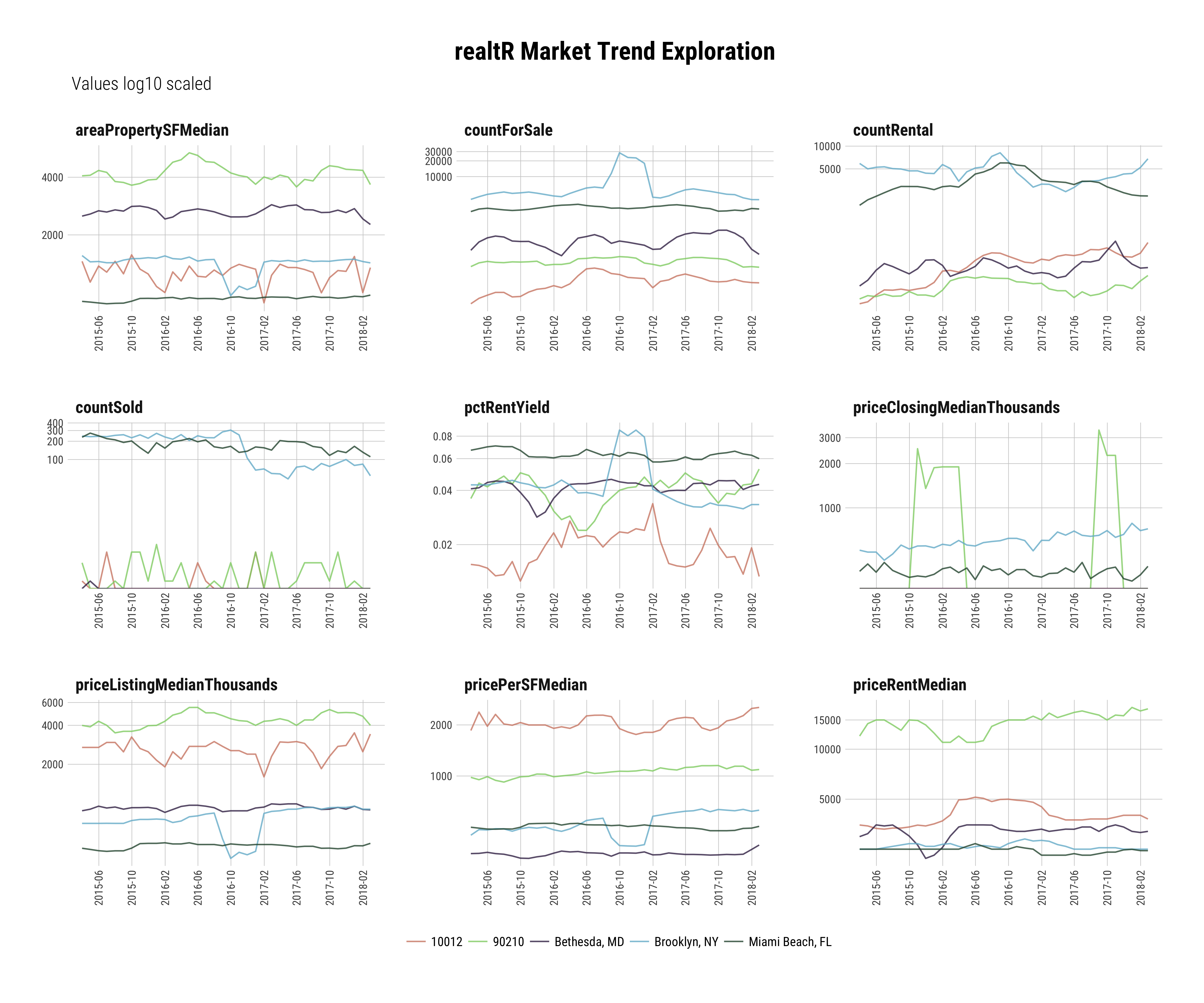

It probably is quickly apparent this visualization contains ALOT of information.

The purpose of this tutorial isn’t data interpretation but I will say this, over last few months there has been a real slow down through out New York City and you can see that in the two New York markets I included, the zip code 10012 and Brooklyn.

The trends() function helps you easily and programmatically access the current and historic market information central to formulating an understanding of an area.

Median Prices

Next up, median_prices.

This is a variant of trends that returns a subset of median price related data from the the most recent month.

This function allows you to get a quick, high-level snapshot of your specified locations.

The median_price function only accepts a city/state location input.

I am going to demonstrate the function by exploring a few of the country’s ritziest vacation home markets.

ritzy_beach_towns <-
  c(
    "East Hampton, NY",
    "Quogue, NY",
    "Bethany Beach, DE",
    "Nantucket, MA",
    "Vineyard Haven, MA",
    "Haleiwa, HI",
    "Kennebunkport, ME",
    "Montauk, NY",
    "Water Mill, NY"
  )
df_median_ritzy <- 
  median_prices(locations = ritzy_beach_towns,
                return_message = F)

Once the data is acquired its easy to explore it.

I’m going to examine median price per square foot explained by median listing price, grouped by state, sized by median property area.

Sounds like this could visualization overkill but as you will see, when using a labeled interactive visualization it ends up being quite insightful.

df_median_ritzy %>%
  arrange(desc(priceListingMedian)) %>%
  hchart(
    "scatter",
    backgroundColor = "#FFFFFF",
    style = list(fontSize = "2em"),
    fontFamily = "Helvetica",
    hcaes(
      x = priceListingMedian,
      y = pricePerSFMedian,
      group = stateSearch,
      size = areaPropertySFMedian
    )
  )  %>%
  hc_add_theme(hc_theme_smpl()) %>%
  hc_plotOptions(series = list(
    dataLabels = list(
      enabled = TRUE,
      inside = TRUE,
      format = '{point.locationSearch}',
      color = 'black',
      padding = 0,
      font = '8px'
    )
  )) %>%
  hc_title(text = "Ritzy Vacation Market Median Price Exploration") %>%
  hc_subtitle(text = "Price PSF by Listing Price Sized by Home Area<br>Data As Of: 2018-03", align = "left") %>%
  hc_legend(
    layout = "vertical",
    verticalAlign = "top",
    align = "right",
    valueDecimals = 0
  )

Looks like if you want to join all the cool kids in Montauk you need some serious cash and an ability to make due with a fairly small property.

Contrast that with nearby-sh Quoque which, though nominally more expensive on average, gets you, as they say in real estate speak, much more home per pound.

Vitality

The final market market function I am going to examine is vitality.

This returns real time information centered around meta-listing data including but not limted to the number of active sales, rentals, recently sold properties, and new listings.

It also returns the four most recent listings for each search location in a nested data frame.

Unlike median_prices this function accepts a variety of location inputs including:

City and State

County and State

Neighborhood, City and State

Zip code

To demonstrate the function I am going to layer in some additional locations to the ritzy vacation markets from the last search. They include two San Francisco zip codes and a couple of prominent east coast neighborhoods.

sf_zips <-
  c(94123, 94133)
  
random_ec_hoods <-
  c(
    "Federal Hill, Baltimore, MD",
    "Cleveland Park, Washington, DC",
    "Rittenhouse Square, Philadelphia, PA",
    "Nomad, New York, NY",
    "Beacon Hill, Boston, MA"
  )
  
vitality_locations <-
  c(ritzy_beach_towns,
    random_ec_hoods,
    sf_zips)

  df_vitality <-
    vitality(locations = vitality_locations,
             return_message = F)

Now after nesting the data by search location we can explore the results in JSON.

df_vitality %>%
  nest(-locationSearch, .key = 'dataSearch') %>% 
  listviewer::jsonedit()

Now I am going use this data to build a dot-plot of inventory by location to try to try to get an idea of supply dynamics.

Like one of our prior examples, there is wide variance in the data which can make a visualization harder to interpret without adjustments.

This time, instead of taking the log10, value axis will reflect the square root of the value variable.

df_vitality %>%
  select(countForSale, locationSearch) %>%
  ggplot(aes(x = countForSale, y = fct_reorder(locationSearch, countForSale))) +
  geom_point(color = "#0072B2", size = 3) +
  scale_x_continuous(
    name = "Properties for Sale",
    limits = c(0, 650),
    trans = 'sqrt',
    breaks = scales::pretty_breaks(n = 10),
    expand = c(0, 0)
  ) +
  scale_y_discrete(name = NULL, expand = c(0, 0.5)) +
  theme(
    axis.ticks.length = grid::unit(0, "pt"),
    axis.title = element_text(size = 12),
    plot.margin = margin(7, 21, 7, 7)
  ) +
  hrbrthemes::theme_ipsum_ps(grid="XY", strip_text_face="bold") +
  ggtitle(label = "Inventory by market",
          subtitle = glue::glue("Data as of {Sys.Date()} "))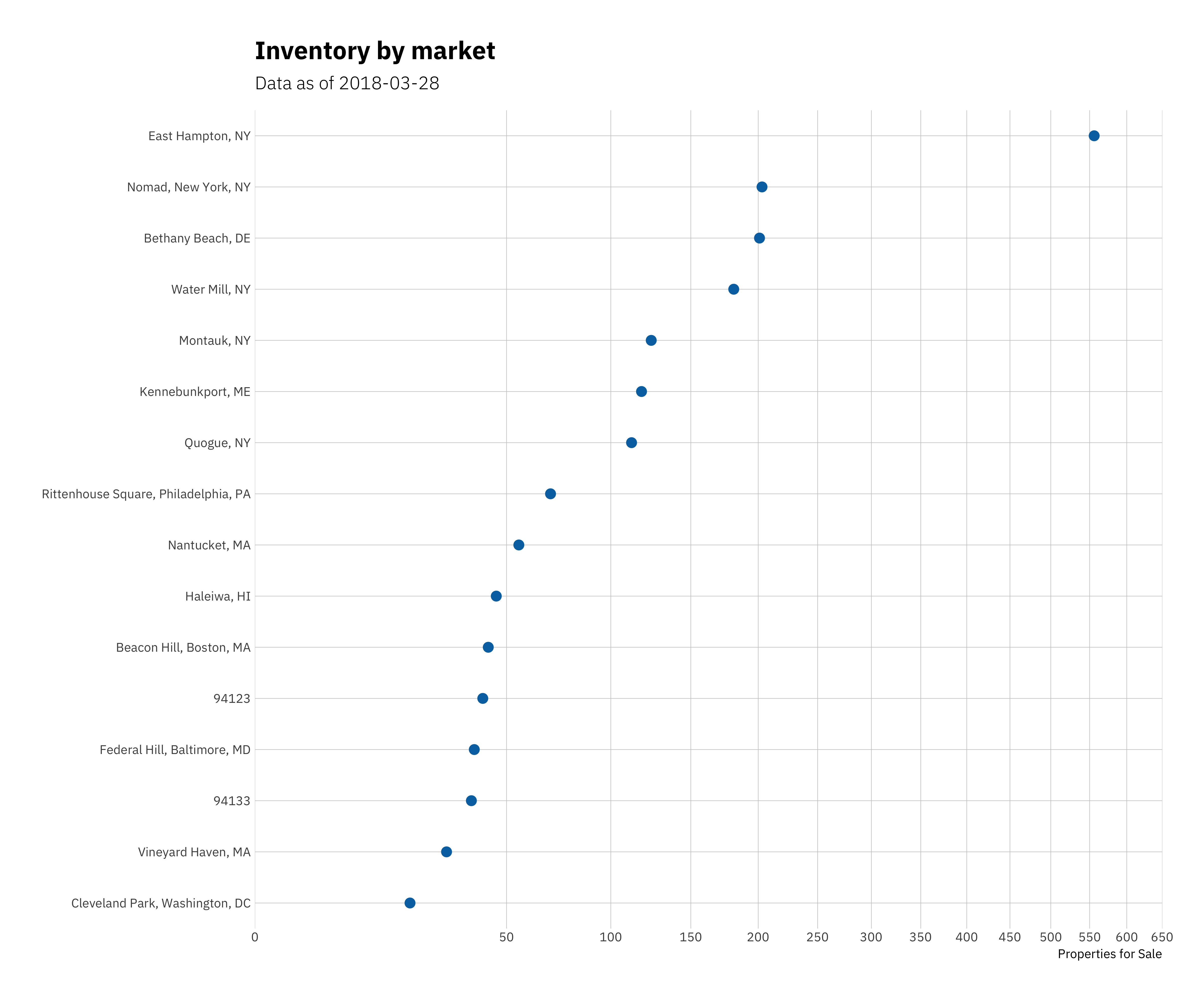

Hmmmmm… looks like now could be an interesting time to start closely watching East Hampton if you enjoy going “Out East” during the hot NYC summers, looks like a pretty sizable amount of supply for a market of its size.

Now I’m going to showcase what I expect will excite people most, real-time access to millions of individual property.

Listings

A minimal understanding of some R basics and realtR will allow anyone to explore updated property listings throughout the United States.

The data includes details on everything from the listing broker, time on market, property features, property size, lot size, age, price, and much more.

Similar to the market-level functions, location is the only required input. The listing family of functions accept a variety location inputs including:

Specified Address

Street Name and City

Neighborhood

City and State

Zip Code

County

Unlike the meta functions, there are additional parameters available to target the search. They include parameters around price, property size, property type, property features, lot area, and property age. If you want to see all of th available inputs you can do so <<a href=“https://asbcllc.com/realtR/reference/listings.html” title=“params”, target=“_blank“>here.

The property types and listing features each a dictionary containing their respective usable inputs.

To isolate these parameters just provide a vector of the desired specifications from the name column.

These are the usable listing features:

realtR::dictionary_listing_features()

and these are the specifiable property types:

realtR::dictionary_property_types()

If you wanted to target only properties central air, a community pool and a fire place you’d pass through a character vector with those selections into the features input in the function.

Here is how to us the function.

I am going to stick with the locations defined earlier in our vitality search but hone in on only newly constructed properties.

df_new_construction_listings <-
  listings(locations = vitality_locations,
         is_new_construction = T)

Lets get a high level view of the results using the fantastic skim() function.

df_new_construction_listings %>%
  skimr::skim()

## Skim summary statistics
##  n obs: 53 
##  n variables: 33 
## 
## Variable type: character 
##               variable missing complete  n min max empty n_unique
##        addressProperty       0       53 53   4  29     0       53
##           cityProperty       0       53 53   6  13     0       20
##         locationSearch       0       53 53   5  36     0       14
##          nameBrokerage      26       27 53   7  53     0       15
##           nameLocation       0       53 53   5  34     0       14
##  nameLocationValidated       0       53 53   5  39     0       14
##           slugLocation       0       53 53   5  37     0       14
##              slugState       0       53 53   2   2     0        9
##          stateProperty       0       53 53   2   2     0        9
##          statusListing      44        9 53   3  15     0        3
##         statusProperty       0       53 53   8   8     0        2
##    statusPropertyBuild      48        5 53  14  14     0        1
##             typeGarage      30       23 53   5   5     0        5
##            typeListing       0       53 53  14  29     0        2
##           typeProperty      48        5 53   8   8     0        1
##             typeSearch       0       53 53   4   4     0        1
##               urlImage      16       37 53  87  89     0       37
##             urlListing       0       53 53  88 144     0       53
##        zipcodeProperty       0       53 53   5   5     0       19
## 
## Variable type: logical 
##           variable missing complete  n mean          count
##        hasPendings       0       53 53    1 TRU: 53, NA: 0
##  isNewConstruction       0       53 53    1 TRU: 53, NA: 0
## 
## Variable type: numeric 
##           variable missing complete  n       mean          sd        p0
##        areaLotSize      24       29 53   35328.31 28760.91      3920   
##     areaPropertySF       2       51 53    3273.61  2197.69       488   
##         countBaths       0       53 53       3.23     1.6          1   
##     countBathsFull      10       43 53       3.53     1.59         1   
##     countBathsHalf      19       34 53       1.18     0.46         1   
##          countBeds       0       53 53       3.49     1.72         0   
##   latitudeProperty       2       51 53      39.03     5.35        21.34
##  longitudeProperty       2       51 53     -83.64    25.68      -158.1 
##      numberListing       0       53 53       3.83     2.97         1   
##       priceListing       5       48 53 5400304.1      1.1e+07 365000   
##  pricePerSFListing       7       46 53    1467.71  1489.41       213.62
##       sizeLotAcres      24       29 53     676.69  2116.37         0.25
##        p25     median        p75         p100     hist
##   20473      23522      44000    126427       ▃▇▃▁▁▁▁▁
##    1476       3009       4803     10079       ▇▃▅▆▂▁▁▁
##       2          3          4         7       ▃▇▇▅▁▃▁▂
##       2          3          4.5       7       ▂▆▇▅▁▃▁▂
##       1          1          1         3       ▇▁▁▁▁▁▁▁
##       2          3          5         7       ▁▃▆▇▃▅▂▂
##      39.1       40.75      41.02     43.47    ▁▁▁▁▁▁▂▇
##     -75.12     -73.98     -72.2     -70.44    ▁▁▁▁▁▁▁▇
##       2          3          5        12       ▇▃▃▁▁▂▁▁
##  747250    3365000    5174750         7.4e+07 ▇▁▁▁▁▁▁▁
##     482.12     741.46    2298.44   7322.15    ▇▂▂▁▁▁▁▁
##       0.51       0.71       1.14   8276       ▇▁▁▁▁▁▁▁

Here are the individual listings in table form.

df_new_construction_listings

Now I am going to explore the distribution of listing price per square foot by after excluding any NA values.

library(ggbeeswarm)
df_new_construction_listings %>%
  filter(!is.na(pricePerSFListing)) %>%
  ggplot(aes(pricePerSFListing, locationSearch, color = typeListing)) +
  geom_quasirandom(groupOnX = F) +
  guides(colour = guide_legend(nrow = 1),
         guide = guide_legend(title = NULL)) +
  labs(
    x = "Listing Price Per SF",
    y = "",
    title = "New Construction Pricing",
    subtitle = "Data as of March 2018",
    caption = "data via realtR",
    color = ""
  ) +
  scale_x_continuous(breaks = scales::pretty_breaks(n = 15),
                     labels = scales::dollar) +
  viridis::scale_color_viridis(discrete = TRUE, option = "D") +
  hrbrthemes::theme_ipsum_rc(grid="XY", strip_text_face="bold") +
  theme(legend.position = "bottom", legend.direction = "vertical")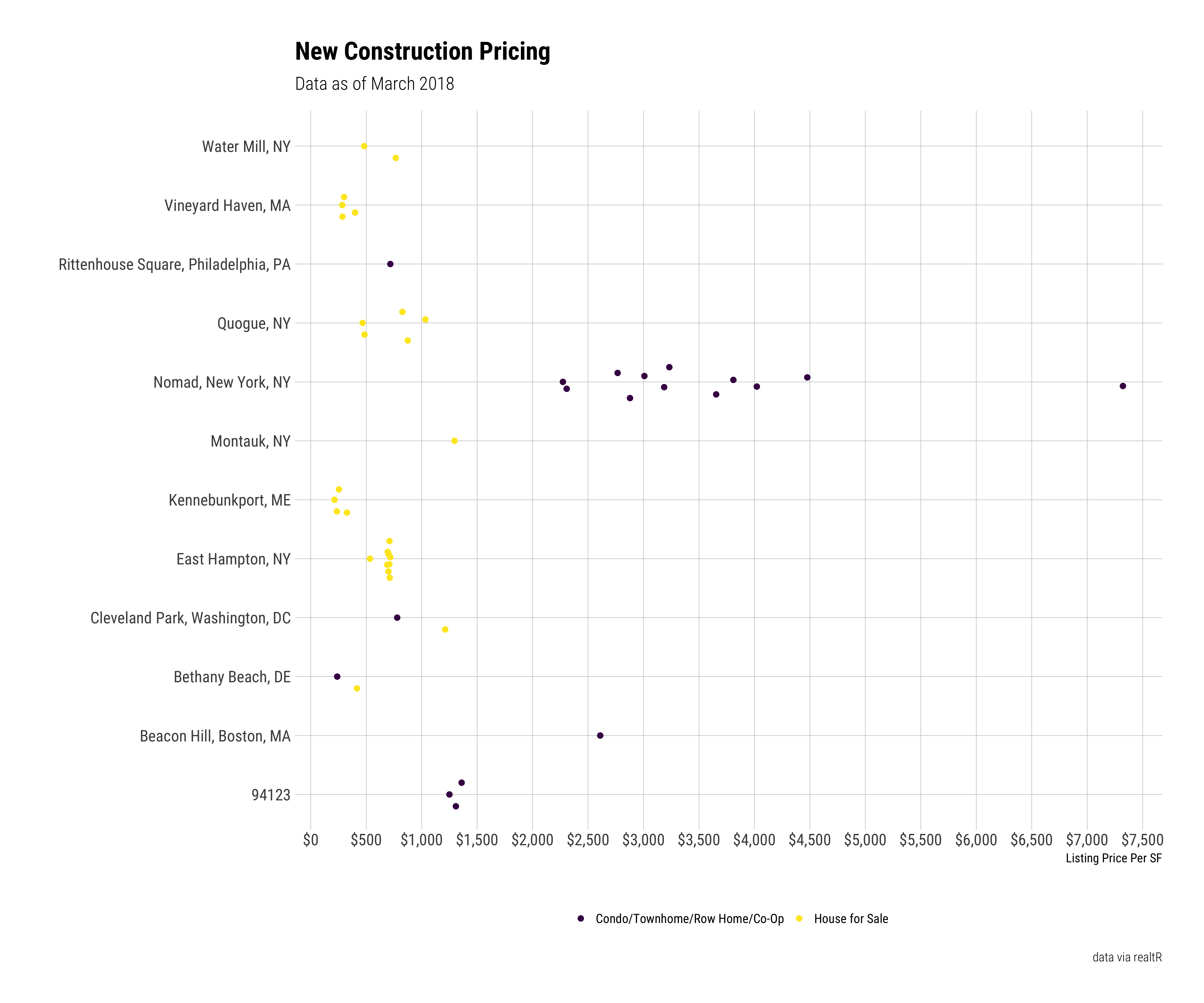

MAN Nomad, and frankly all of New York city, is expensive!!

That’s what happens when you have a nearly decade long leveraged fueled real estate bubble.

Ridiculous asking prices are a direct bi-product developers using other peoples’ money to massively over pay for land assuming a never ending trend of near double digit price growth for newly constructed condos. The real world doesn’t always work like this.

It will be interesting to see if the New York properties, especially those asking more than $2500 PSF end up selling any where near their current prices.

Time will tell and realtR will help me easily keep track!

Going a Step Further with Listing Details

The base listing function family [listings(), map_listings(), properties_nearby()] all return a sizable amount of information but sometimes you may need more. That is what the parse_listing_urls function does for you.

After feeding it a vector listing urls and it will return all the information contained from the actual listings including:

Detailed brokerage information

Property features

Neighborhood information

School information

Prior listing history

Property taxes

Outbound urls

Much of the data returned is nested and so to fully maximize use of this function it is important to understand how to work with nested data in R.

This information returned by this function is extremely useful for advanced modeling, sophisticated visualizations, image processing, text analysis and geo-spatial exploration.

In the next and final section I will demonstrate how to use this function to get additional data that will allow us to build a sophisticated trelliscope and interactive map.

The trelliscope is built using function from one of my private packages so I challenge anyone who is intrigued by the output to invest a bit of time learning Ryan Hafen’s <a href=“https://github.com/hafen/trelliscopejs/” title=“trelli”, target=“_blank“>trelliscopeJS package.

There is good documentation <a href=“http://ryanhafen.com/blog/pokemon” title=“ryan_blog”, target=“_blank“>on his blog about how to build image panel trelliscopes like the one I am about to use.

Advanced Listing Data

The data from our listings() contains the only required input to use the parse_listing_urls function, listing urls.

All you need to do is pass through a vector containing the urls you wish to acquire more information about and realtR does the rest.

For this search we will look up all of the matched results.

df_detailed_listings <-
  df_new_construction_listings$urlListing %>%
  parse_listing_urls()

Lets skim this data:

df_detailed_listings %>% skimr::skim()

## Skim summary statistics
##  n obs: 53 
##  n variables: 37 
## 
## Variable type: character 
##            variable missing complete  n min  max empty n_unique
##     addressProperty       0       53 53  10   29     0       51
##        cityProperty       0       53 53   6   13     0       20
##     descriptionText       0       53 53 253 5531     0       51
##           nameAgent       5       48 53  10   19     0       30
##       nameBrokerage      26       27 53   7   53     0       15
##       stateProperty       0       53 53   2    2     0        9
##       statusListing       0       53 53   6   22     0        5
##           styleHome      18       35 53   4   19     0       18
##  typePropertyDetail       0       53 53  18   29     0        2
##            urlImage       3       50 53  87   90     0       50
##          urlListing       0       53 53  88  144     0       53
##           urlVRTour      45        8 53  24   75     0        7
##     zipcodeProperty       0       53 53   5    5     0       19
## 
## Variable type: Date 
##  variable missing complete  n        min        max     median n_unique
##  dateData       0       53 53 2018-03-27 2018-03-27 2018-03-27        1
## 
## Variable type: list 
##            variable missing complete  n n_unique min_length median_length
##           dataComps       0       53 53       53          4             7
##  dataListingHistory       0       53 53       45          0             4
##    dataNeighborhood       0       53 53       20          0             6
##          dataPhotos       0       53 53       51          0             1
##          dataSchool       0       53 53       27          0             4
##           dataTaxes       0       53 53       15          0             0
##  max_length
##           7
##           4
##           8
##           1
##           4
##           3
## 
## Variable type: logical 
##           variable missing complete  n mean                   count
##           hasComps       0       53 53 1             TRU: 53, NA: 0
##  hasListingHistory       0       53 53 0.83  TRU: 44, FAL: 9, NA: 0
##    hasNeighborhood       0       53 53 0.87  TRU: 46, FAL: 7, NA: 0
##          hasPhotos       0       53 53 0.94  TRU: 50, FAL: 3, NA: 0
##         hasSchools       0       53 53 0.92  TRU: 49, FAL: 4, NA: 0
##           hasTaxes       0       53 53 0.26 FAL: 39, TRU: 14, NA: 0
## 
## Variable type: numeric 
##            variable missing complete  n     mean       sd        p0
##      areaPropertySF       2       51 53  3273.61  2197.69    488   
##          countBaths       0       53 53     3.23     1.6       1   
##           countBeds       0       53 53     3.49     1.72      0   
##          countComps       0       53 53    21        0        21   
##  countDaysOnRealtor       0       53 53    88.43   105.3       1   
##       countListings       9       44 53     4.93     8.45      1   
##         countPhotos       3       50 53    14.52     9.01      2   
##        priceListing       0       53 53 5e+06    1e+07    365000   
##   pricePerSFListing       2       51 53  1394.89  1435.48    213.62
##        sizeLotAcres      24       29 53   676.69  2116.37      0.25
##           yearBuilt       9       44 53  2003.18    36.66   1912   
##        p25     median        p75        p100     hist
##    1476       3009       4803    10079       ▇▃▅▆▂▁▁▁
##       2          3          4        7       ▃▇▇▅▁▃▁▂
##       2          3          5        7       ▁▃▆▇▃▅▂▂
##      21         21         21       21       ▁▁▁▇▁▁▁▁
##      29         40        113      433       ▇▁▁▁▁▁▁▁
##       1          2          5.25    52       ▇▁▁▁▁▁▁▁
##       8         12         20       41       ▃▇▅▅▂▁▁▁
##  739000    3295000    4795000        7.4e+07 ▇▁▁▁▁▁▁▁
##     482.87     716.77    1859.35  7322.15    ▇▂▁▁▁▁▁▁
##       0.51       0.71       1.14  8276       ▇▁▁▁▁▁▁▁
##    2017       2018       2018     2018       ▁▁▁▁▁▁▁▇

As I mentioned early there are lots of features including a host of nested ones, I am going to look at 5 random detailed listings so we can see what that looks like

df_detailed_listings %>% 
  sample_n(5)

## # A tibble: 5 x 37
##   dateData   countDaysOnRealt… statusListing styleHome  typePropertyDetail
##   <date>                 <dbl> <chr>         <chr>      <chr>             
## 1 2018-03-27               47. Active        Craftsman  Single family home
## 2 2018-03-27              154. Active        Federal    Condo/townhome/ro…
## 3 2018-03-27               25. New Listing   Post Mode… Single family home
## 4 2018-03-27               80. Active        Colonial … Single family home
## 5 2018-03-27               22. Active        <NA>       Condo/townhome/ro…
## # ... with 32 more variables: yearBuilt <dbl>, urlImage <chr>,
## #   dataPhotos <list>, countPhotos <dbl>, addressProperty <chr>,
## #   cityProperty <chr>, stateProperty <chr>, zipcodeProperty <chr>,
## #   nameAgent <chr>, nameBrokerage <chr>, priceListing <dbl>,
## #   dataNeighborhood <list>, descriptionText <chr>, areaPropertySF <dbl>,
## #   countBaths <dbl>, countBeds <dbl>, sizeLotAcres <dbl>,
## #   dataListingHistory <list>, countListings <dbl>, dataComps <list>,
## #   countComps <dbl>, dataSchool <list>, urlListing <chr>,
## #   dataTaxes <list>, urlVRTour <chr>, pricePerSFListing <dbl>,
## #   hasComps <lgl>, hasTaxes <lgl>, hasPhotos <lgl>, hasSchools <lgl>,
## #   hasNeighborhood <lgl>, hasListingHistory <lgl>

One important thing to remember is that there are some overlapping columnslistings() where the data returned by parse_listing_urls may not match that returned by listings, map_listings or properies_near. The data returned from the parse_listing_urls function is the best authority on accuracy so I like to remove the matching columns from the listing results and join in the new data from the listing urls.

I will demonstrate how to do this to build the final two visualizations.

df_all <-
  df_detailed_listings %>%
  select(-one_of(
    c(
      "statusListing",
      "urlImage",
      "addressProperty",
      "cityProperty",
      "stateProperty",
      "zipcodeProperty",
      "priceListing",
      "areaPropertySF",
      "countBaths",
      "countBeds",
      "sizeLotAcres",
      "nameBrokerage",
      "pricePerSFListing"
    )
  )) %>%
  left_join(df_new_construction_listings)

## Joining, by = "urlListing"

I need a photo to feature in both of my visualizations. The listings function will sometimes return a photo but not in every case. Most listing urls contain at least a single photo so I am going to pick a random photo from the detailed data and use that as the property url if there isn’t already one from the listings search.

df_all <-
  df_all %>%
  mutate(idRow = 1:n()) %>%
  left_join(
    df_detailed_listings %>%
      mutate(idRow = 1:n()) %>%
      filter(hasPhotos) %>%
      dplyr::select(idRow, dataPhotos) %>%
      unnest() %>%
      group_by(idRow) %>%
      sample_n(1) %>%
      ungroup()
  ) %>%
  select(-idRow) %>%
  suppressMessages()

df_all <-
  df_all %>%
  mutate(urlImage = case_when(is.na(urlImage) ~ urlPhotoProperty,
                              TRUE ~ urlImage))

Next I am going select a portion joined data of the information to build to power the interactive trelliscope I mentioned early.

df_all <-
  df_detailed_listings %>%
  select(-one_of(
    c(
      "statusListing",
      "urlImage",
      "addressProperty",
      "cityProperty",
      "stateProperty",
      "zipcodeProperty",
      "priceListing",
      "areaPropertySF",
      "countBaths",
      "countBeds",
      "sizeLotAcres",
      "nameBrokerage",
      "pricePerSFListing"
    )
  )) %>%
  left_join(df_new_construction_listings)

df_all <-
  df_all %>%
  mutate(idRow = 1:n()) %>%
  left_join(
    df_detailed_listings %>%
      mutate(idRow = 1:n()) %>%
      filter(hasPhotos) %>%
      dplyr::select(idRow, dataPhotos) %>%
      unnest() %>%
      group_by(idRow) %>%
      sample_n(1) %>%
      ungroup()
  ) %>%
  select(-idRow) %>%
  suppressMessages()

df_all <-
  df_all %>%
  mutate(urlImage = case_when(is.na(urlImage) ~ urlPhotoProperty,
                              TRUE ~ urlImage))

Now I can use this data to power a trelliscope.

The trelliscope is a great way to explore, filter and examine tabular data. It works across devices, allows links and is super fast. Go ahead, click the filter button and start drilling down on questions of interest!

df_all %>%
  select(-matches("^has|^data")) %>%
  plot_image_trelliscope(
    image_column = "urlImage",
    id_columns = list(
      is_except = FALSE,
      columns = c(
        "nameLocationValidated",
        "addressProperty",
        "slugState",
        "cityProperty",
        "styleHome",
        "priceListing",
        "pricePerSFListing",
        "areaPropertySF",
        "zipcodeProperty"
      ),
      regex = NULL
    ),
    title = "New_Construction_Trelliscope",
    trelliscope_parameters = list( = 
      rows = 1,
      columns = 3,
      path = NULL
    )
  )

You can view a full-screen version here.

Finally, I am going to use leaflet javascript library to build an interactive map with customizable layers. The map will contain a super imposed property photo at each latitude and longitude. I also going to use a bit of javascript to build some click-able summary clusters that show a count of the number of the number of properties in your search area, it will adjust as you zoom in and out. I also am a sucker for cool layers so I am going to let you explore a couple of the nearly 100 layers leaflet lets you select to power a map!

You can view a stand-alone version here.

This map just scratches the surface of what you can do. With a couple of additional steps you can overlay additional property information and much more

Closing Thoughts

There are a couple of other functions that I didn’t go over but they work in a similar manner and if you have any issues please file an issue on Github.

Thinking back on one of my favorite shows growing up, GI JOE, they used to end each show with a message centered around this:

When dealing with the sharks of the real estate brokerage world knowing is far than half the battle, probably some where close to 98% of the battle! realtR mixed with a bit of coding skills, some street smarts and a heavy dose of skepticism when dealing with an agent will arm you for victory.

I hope you enjoy using the package as much as I have had building it.

Until next time.